
crime <- read.csv("crime.csv")
crime <- crime[-c(9293:9302),]
The data is arranged as one giant merged cell for each state with many rows representing cities within it
str(crime)
which(crime$State != "")
library(zoo)
States <- (crime$State)
States[States == ""] <- NA
States <- na.locf(States, na.rm = TRUE, fromLast = FALSE)
crime$States <- States
crime <- crime[,-c(1)]
crime <- crime[,-c(14:16)]

crime[is.na(crime)] <- 0
For now we’re more interested in crime at the state level rather than city
crimeAgg <- aggregate(. ~ States, data = crime, sum)
crimeAgg$ViolentPerCap <- (crimeAgg$Violent.crime / crimeAgg$Population) * 100
crimeAgg$BurglaryPerCap <- (crimeAgg$Burglary / crimeAgg$Population) * 100
crimeAgg$VehiclePerCap <- (crimeAgg$Motor.vehicle.theft / crimeAgg$Population) * 100
Preliminarily, we can examine crime by state in ggplot2
library(ggplot2)
ggplot(crimeAgg, aes(x=States, y=VehiclePerCap)) + geom_col()
ggplot(crimeAgg, aes(x=States, y=ViolentPerCap)) + geom_col()
ggplot(crimeAgg, aes(x=States, y=BurglaryPerCap)) + geom_col()
library(choroplethr)
library(choroplethrMaps)
violentCrime <- crimeAgg[,-c(2:14,16, 17, 18)]
colnames(violentCrime) <- c("region", "value")
violentCrime$region <- sapply(violentCrime$region, tolower)
violentCrime$value <- as.numeric(as.character(violentCrime$value))
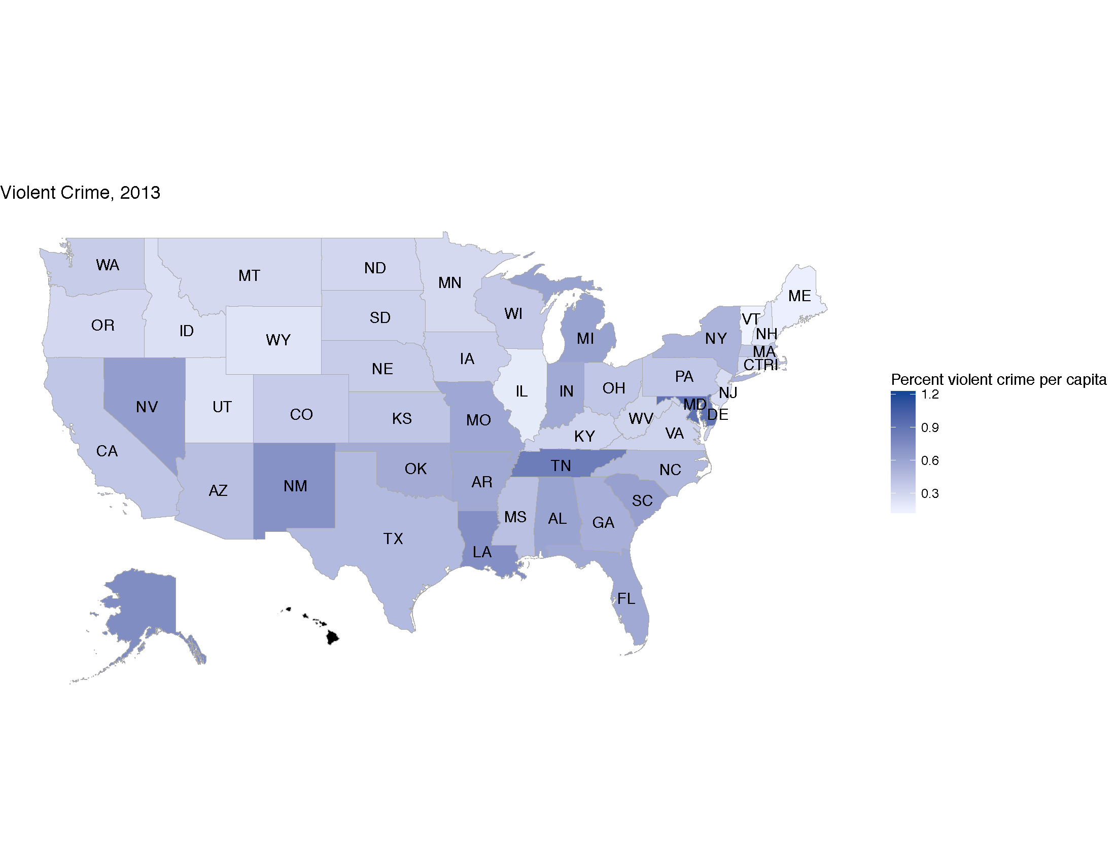
state_choropleth(violentCrime, title = "Violent Crime, 2013", legend =
"Percent violent crime per capita", num_colors = 1, reference_map = FALSE)

 https://github.com/tracybedrosian/Choropleth-2013-Crime-in-America
Leave a Reply